A Journey of Generative Model

Generating illustrations or photorealistic images with natural language instructions is no longer surprising today. We can now generate high-quality images with a lot of AI-based tools, such as DALL-E, Stable Diffusion, Midjourney, and many more. Technology that makes these possible is the Generative Model. Generative models learn how data are generated and then generate new (pseudo) data that looks similar to the existing (human-generated) ones. For example, ChatGPT generates the following images.

In this article, we aim to walk you through the mathematical concept of the Generative Model, starting from Normal Distribution, stepping up to Latent Variable Model with VAE as a case study. Finally, we will introduce Diffusion Model, a representative one that amazes the world with its realistic, high-quality image generation capability.

Generative Model

The objective of a generative model is to represent (modeling) the distribution \(p(x)\) of observed data \(x\). Once the distribution \(p(x)\) is obtained, new (pseudo) data can be generated (sampling) from that distribution.

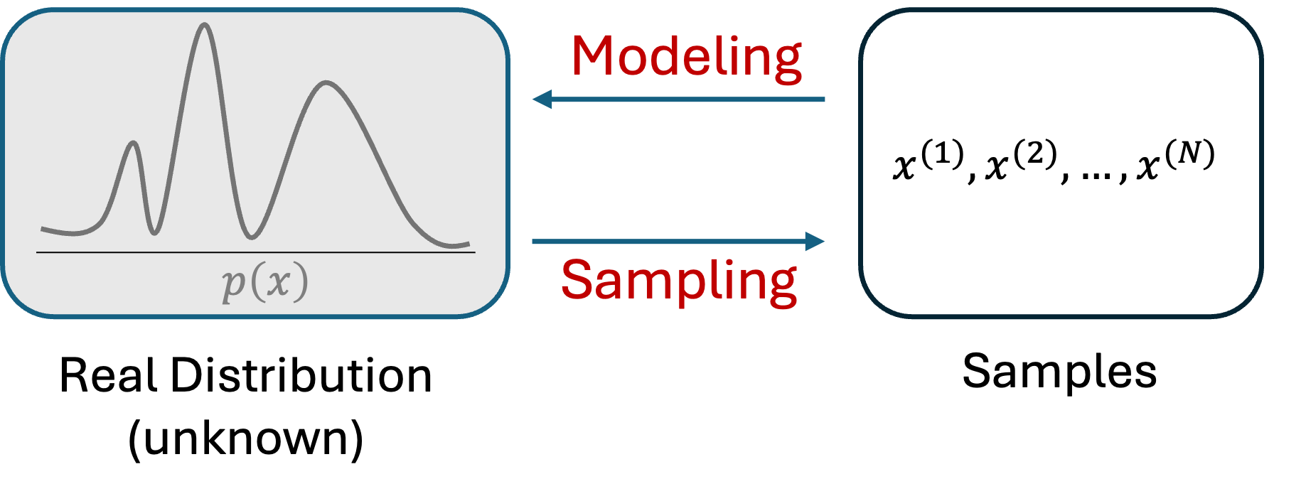
Ideally, if we obtain the actual distribution, we could quickly generate new, accurate data. Unfortunately, in reality, it is impossible to get such actual distribution. In such a scenario, we use some limited numbers of samples to estimate the actual distribution. This can be implemented with the following two processes:

• Modeling: We assume a probabilistic distribution can approximate the actual distribution.

• Parameter Estimation: We adjust the parameters of that probabilistic distribution to make the distribution fit with the samples we have in hand. A method used for this estimation is Maximum Likelihood Estimation.

Modeling

Modeling in generative models involves creating a mathematical representation of the data’s distribution. This is critical as it allows the model to encapsulate the essential traits and variability of the data. Depending on the type and complexity of the data, the modeling approach varies significantly.

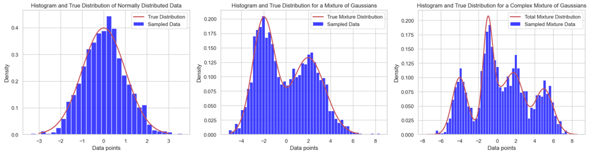
Example with 1D Data: Normal Distribution

For one-dimensional (1D) data, a simple probabilistic model like the normal distribution can be practical. Consider a set of measurements centered around a specific value with a certain amount of random deviation (e.g., the heights of adult males). A normal distribution, defined by its mean (\(\mu\)) and variance (\(\sigma^2\)), can model this data efficiently. This approach is straightforward yet powerful in capturing data’s central tendency and dispersion.

Expanding to High-Dimensional Data: Images and Language

As the dimensionality and complexity of data increase, more sophisticated models are required. For image data, convolutional neural networks (CNNs) are typically used to model the spatial hierarchies and dependencies between pixels, capturing features from edges to complex objects within an image. In the case of sequential data such as text or time series, models like recurrent neural networks (RNNs) or transformers are employed. These models can handle temporal dynamics and long-range dependencies, making them suitable for language translation or speech recognition tasks.

Parameter Estimation

The parameter estimation process involves fine-tuning the model’s parameters to fit the data closely. Maximum Likelihood Estimation (MLE) is commonly used to achieve this by maximizing the likelihood function, indicating how likely the observed data is under the assumed model.

Example with 1D Data: Normal Distribution

For a normal distribution modeling 1D data, MLE would determine the mean and variance that maximize the likelihood of observing the sample data. This process involves calculating the average and the spread of the data points around that average, which are straightforward yet effective parameter estimations.

Expanding to High-Dimensional Data: Images and Language

Parameter estimation becomes more intricate in complex scenarios like images or language. Techniques such as gradient descent are used to adjust the weights in neural networks. These techniques iteratively reduce the error between the model’s predictions and the actual data, adjusting parameters like filter weights in CNNs or attention weights in transformers.

Show code cell source Hide code cell source

import numpy as np
import matplotlib.pyplot as plt
import seaborn as sns
from matplotlib.animation import FuncAnimation
from IPython.display import HTML, display

# Generate some dummy data
np.random.seed(42)
data = np.concatenate([
    np.random.normal(-2, 1, 300),
    np.random.normal(2, 1, 300)
])
data = data.reshape(-1, 1)  # Reshape to fit our needs

# Number of components
K = 2

# Initialize parameters
means = np.array([1, 2], dtype=np.float64)  # Initial guesses for means
covariances = np.array([1.5, 1.5], dtype=np.float64)  # Initial guesses for variances
weights = np.array([0.5, 0.5], dtype=np.float64)  # Initial guesses for mixing coefficients

# Plotting setup
fig, ax = plt.subplots()
x = np.linspace(-6, 6, 1000)

def update(frame):
    global means, covariances, weights

    # E-step: Calculate responsibilities
    responsibilities = np.zeros((data.shape[0], K))
    for k in range(K):
        likelihood = np.exp(-0.5 * ((data - means[k])**2) / covariances[k]) / np.sqrt(2 * np.pi * covariances[k])
        responsibilities[:, k] = weights[k] * likelihood.ravel()
    responsibilities /= responsibilities.sum(axis=1, keepdims=True)

    # M-step: Update parameters
    Nk = responsibilities.sum(axis=0)
    weights = Nk / Nk.sum()
    means = (data.T @ responsibilities / Nk).ravel()
    covariances = np.array([(responsibilities[:, k] * (data.flatten() - means[k])**2).sum() / Nk[k] for k in range(K)])

    # Clear the plot and replot the data histogram
    ax.clear()
    sns.histplot(data.ravel(), bins=30, kde=False, color="white", ax=ax, stat='density')
    
    # Plotting each component
    for k in range(K):
        pdf = weights[k] * np.exp(-(x - means[k])**2 / (2 * covariances[k])) / np.sqrt(2 * np.pi * covariances[k])
        ax.plot(x, pdf, label=f'Component {k+1}')
    
    ax.set_xlim(-6, 6)
    ax.set_ylim(0, 0.3)
    ax.legend()
    ax.set_title(f'EM Iteration: {frame + 1}')

ani = FuncAnimation(fig, update, frames=20, repeat=False)
plt.close(fig)  # Prevent display of static plot

# Render the animation as HTML
html_str = ani.to_jshtml()
display(HTML(html_str))

Once Loop Reflect